[Vision] Image Segmentation (이미지 분할)

이번 포스팅에서는 Image segmentation에 대해서 실습해보도록 하겠습니다.

Image segmentation은 이미지에서 개체가 있는 위치, 해당 개체의 모양, 그리고 어떤 픽셀이 어떤 객체에 속하는 지를 분류하는 Task입니다.

즉 다시 말해서, 이미지 전체를 여러가지 class로 분류하겠다는 것입니다.

​​

1. 사용할 패키지 불러오기.

import tensorflow as tf
from tensorflow_examples.models.pix2pix import pix2pix

import tensorflow_datasets as tfds
tfds.disable_progress_bar()

from IPython.display import clear_output
import matplotlib.pyplot as plt

import를 활용하여 사용할 패키지를 불어왔습니다.

 

2. 데이터 불러오기.

 

이번 실습에서 사용할 데이터는 Oxford-IIIT 데이터셋입니다.

해당 데이터셋의 이미지에 속하는 픽셀들은 총 3가지분류를 가집니다.

- Class 1: 애완동물에 속한 픽셀

- Class 2: 애완동물과 인접한 픽셀

- Class 3: 위의 두 가지에 해당하지 않는 주변 픽셀

 

dataset, info = tfds.load('oxford_iiit_pet:3.*.*', with_info=True)

 

이미지 전처리를 진행하도록 하겠습니다.

(1) 이미지 Resize

(2) 이미지 Augmentation (좌우 대칭)

(3) 픽셀의 값을 0~1로 Normalize

 

def normalize(input_image, input_mask):
  input_image = tf.cast(input_image, tf.float32) / 255.0
  input_mask -= 1
  return input_image, input_mask

@tf.function
def load_image_train(datapoint):
  input_image = tf.image.resize(datapoint['image'], (128, 128))
  input_mask = tf.image.resize(datapoint['segmentation_mask'], (128, 128))

  if tf.random.uniform(()) > 0.5:
    input_image = tf.image.flip_left_right(input_image)
    input_mask = tf.image.flip_left_right(input_mask)

  input_image, input_mask = normalize(input_image, input_mask)

  return input_image, input_mask

 

Test 데이터셋에 대해서는 (1)과 (3)만 진행하겠습니다.

 

def load_image_test(datapoint):
  input_image = tf.image.resize(datapoint['image'], (128, 128))
  input_mask = tf.image.resize(datapoint['segmentation_mask'], (128, 128))

  input_image, input_mask = normalize(input_image, input_mask)

  return input_image, input_mask

 

그리고 배치사이즈만큼 데이터를 쪼개도록 하겠습니다.

 

TRAIN_LENGTH = info.splits['train'].num_examples
BATCH_SIZE = 64
BUFFER_SIZE = 1000
STEPS_PER_EPOCH = TRAIN_LENGTH // BATCH_SIZE

train = dataset['train'].map(load_image_train, num_parallel_calls=tf.data.experimental.AUTOTUNE)
test = dataset['test'].map(load_image_test)

train_dataset = train.cache().shuffle(BUFFER_SIZE).batch(BATCH_SIZE).repeat()
train_dataset = train_dataset.prefetch(buffer_size=tf.data.experimental.AUTOTUNE)
test_dataset = test.batch(BATCH_SIZE)

 

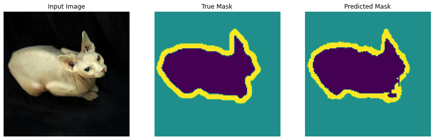
데이터를 한 번 확인해보도록 하겠습니다.

 

def display(display_list):
  plt.figure(figsize=(15, 15))

  title = ['Input Image', 'True Mask', 'Predicted Mask']

  for i in range(len(display_list)):
    plt.subplot(1, len(display_list), i+1)
    plt.title(title[i])
    plt.imshow(tf.keras.preprocessing.image.array_to_img(display_list[i]))
    plt.axis('off')
  plt.show()

for image, mask in train.take(1):
  sample_image, sample_mask = image, mask
display([sample_image, sample_mask])

 

귀여운 토끼가 보이네요!

​

3. 모델 정의

 

이번에 사용할 모델은 U-Net입니다.

U-Net은 Encoder와 Decoder로 나뉘어집니다.

저희는 Encoder로 pre-train 된 MobileNetV2와 Decoder로는 pix2pix모델에서 사용되는 Upsampler를 사용하겠습니다.

​

(1) Encoder

 

base_model = tf.keras.applications.MobileNetV2(input_shape=[128, 128, 3], include_top=False)

# 이 층들의 활성화를 이용합시다
layer_names = [
    'block_1_expand_relu',   # 64x64
    'block_3_expand_relu',   # 32x32
    'block_6_expand_relu',   # 16x16
    'block_13_expand_relu',  # 8x8
    'block_16_project',      # 4x4
]
layers = [base_model.get_layer(name).output for name in layer_names]

# 특징추출 모델을 만듭시다
down_stack = tf.keras.Model(inputs=base_model.input, outputs=layers)

down_stack.trainable = False

 

(2) Decoder

 

up_stack = [
    pix2pix.upsample(512, 3),  # 4x4 -> 8x8
    pix2pix.upsample(256, 3),  # 8x8 -> 16x16
    pix2pix.upsample(128, 3),  # 16x16 -> 32x32
    pix2pix.upsample(64, 3),   # 32x32 -> 64x64
]

 

(3) Full model

 

def unet_model(output_channels):
  inputs = tf.keras.layers.Input(shape=[128, 128, 3])
  x = inputs

  # 모델을 통해 다운샘플링합시다
  skips = down_stack(x)
  x = skips[-1]
  skips = reversed(skips[:-1])

  # 건너뛰기 연결을 업샘플링하고 설정하세요
  for up, skip in zip(up_stack, skips):
    x = up(x)
    concat = tf.keras.layers.Concatenate()
    x = concat([x, skip])

  # 이 모델의 마지막 층입니다
  last = tf.keras.layers.Conv2DTranspose(
      output_channels, 3, strides=2,
      padding='same')  #64x64 -> 128x128

  x = last(x)

  return tf.keras.Model(inputs=inputs, outputs=x)

 

4. 모델 훈련

 

model = unet_model(OUTPUT_CHANNELS)
model.compile(optimizer='adam',
              loss=tf.keras.losses.SparseCategoricalCrossentropy(from_logits=True),
              metrics=['accuracy'])

 

Optimizer로는 가장 많이쓰이는 Adam을 활용하겠습니다.

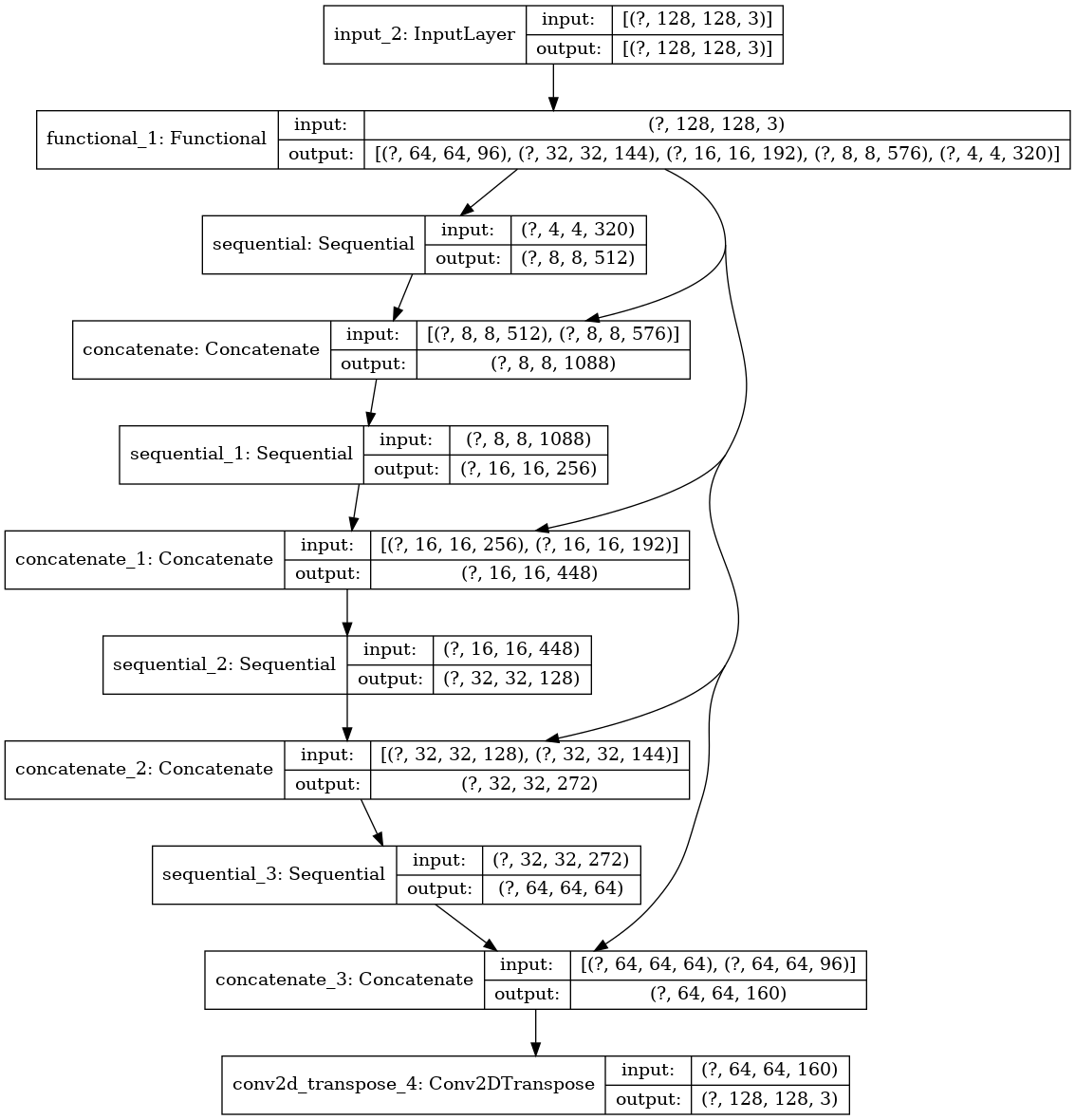
이제 만들어진 모델의 구조를 살펴보겠습니다.

 

tf.keras.utils.plot_model(model, show_shapes=True)

 

한번 예측이 어떻게 나오는지 확인해볼까요?

 

def create_mask(pred_mask):
  pred_mask = tf.argmax(pred_mask, axis=-1)
  pred_mask = pred_mask[..., tf.newaxis]
  return pred_mask[0]

def show_predictions(dataset=None, num=1):
  if dataset:
    for image, mask in dataset.take(num):
      pred_mask = model.predict(image)
      display([image[0], mask[0], create_mask(pred_mask)])
  else:
    display([sample_image, sample_mask,
             create_mask(model.predict(sample_image[tf.newaxis, ...]))])

show_predictions()

 

아직은 잘 안되어있는 모습입니다.

한번 학습을 진행해보도록 하겠습니다.

 

class DisplayCallback(tf.keras.callbacks.Callback):
  def on_epoch_end(self, epoch, logs=None):
    clear_output(wait=True)
    show_predictions()
    print ('\n에포크 이후 예측 예시 {}\n'.format(epoch+1))

EPOCHS = 20
VAL_SUBSPLITS = 5
VALIDATION_STEPS = info.splits['test'].num_examples//BATCH_SIZE//VAL_SUBSPLITS

model_history = model.fit(train_dataset, epochs=EPOCHS,
                          steps_per_epoch=STEPS_PER_EPOCH,
                          validation_steps=VALIDATION_STEPS,
                          validation_data=test_dataset,
                          callbacks=[DisplayCallback()])

 

아까 전의 예시가 놀라운 성능 발전을 이루어 내었습니다.

​

테스트 데이터 셋을 넣어보겠습니다.

 

show_predictions(test_dataset, 3)

 

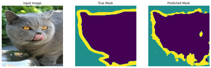
만족스러운 결과를 얻을 수 있었습니다.