728x90
german <- read.csv('German_credit.csv')

colnames(german)

 [1] "ID"                       "Checking_account"         "Duration_in_month"        "Credit_history"
 [5] "Purpose"                  "Credit_amount"            "Saving_accout"            "Present_employment"
 [9] "Installment_rate"         "Personal_status___sex"    "Other_debtors_guarantors" "Present_residence"
[13] "Property"                 "Age"                      "Other_installment_plan"   "Housing"
[17] "Num_of_existing_credits"  "Job"                      "Num_of_people_liable"     "Telephone"
[21] "Foreign_worker"           "Credit_status"

table(german$Credit_status)

  N   Y
700 300
사용할 데이터는 German_credit 데이터셋입니다.
총 1000개의 관측치와 22개의 column으로 구성된 데이터입니다.
저희가 사용할 target 변수는 Credit_status이며, No가 700개, Yes가 300개를 포함합니다.
library(sampling)
stratified_sampling <- strata(german, stratanames = c("Credit_status"), size =c(300,300),
                              method="srswor")

st_data <- getdata(german, stratified_sampling)

table(st_data$Credit_status)

  N   Y
300 300
Class imblance 문제를 완화시키고자, sampling 패키지의 층화추출 함수 strata 를 사용합니다.
데이터 셋은 300개의 No와 300개의 Yes로 구성됩니다.
library(caret)
train <- createDataPartition(st_data$ID, p=0.7, list=FALSE)
td <- st_data[train,]
vd <- st_data[-train,]
다음으로, 데이터 분할을 진행합니다.
Train 데이터셋을 70%, Test 데이터셋을 30%로 분할합니다.
colnames(td)

 [1] "ID"                       "Checking_account"         "Duration_in_month"        "Credit_history"
 [5] "Purpose"                  "Credit_amount"            "Saving_accout"            "Present_employment"
 [9] "Installment_rate"         "Personal_status___sex"    "Other_debtors_guarantors" "Present_residence"
[13] "Property"                 "Age"                      "Other_installment_plan"   "Housing"
[17] "Num_of_existing_credits"  "Job"                      "Num_of_people_liable"     "Telephone"
[21] "Foreign_worker"           "Credit_status"            "ID_unit"                  "Prob"
[25] "Stratum"

td <- td[, -c(1,23,24,25)]
vd <- vd[, -c(1,23,24,25)]
column에 strata 함수에 의해서 생성된 3개가 새롭게 나타납니다.
필요없는 이 3가지 변수와 ID 변수를 제거하였습니다.
td$Job <- as.factor(td$Job)
td$Other_debtors_guarantors <- as.factor(td$Other_debtors_guarantors)
td$Other_installment_plan <- as.factor(td$Other_installment_plan)
td$Personal_status___sex <- as.factor(td$Personal_status___sex)
td$Property <- as.factor(td$Property)
td$Purpose <- as.factor(td$Purpose)
td$Saving_accout <- as.factor(td$Saving_accout)
td$Present_employment <- as.factor(td$Present_employment)

vd$Job <- as.factor(vd$Job)
vd$Other_debtors_guarantors <- as.factor(vd$Other_debtors_guarantors)
vd$Other_installment_plan <- as.factor(vd$Other_installment_plan)
vd$Personal_status___sex <- as.factor(vd$Personal_status___sex)
vd$Property <- as.factor(vd$Property)
vd$Purpose <- as.factor(vd$Purpose)
vd$Saving_accout <- as.factor(vd$Saving_accout)
vd$Present_employment <- as.factor(vd$Present_employment)
그리고, 범주형 변수의 자료형을 factor로 변경해줍니다.
# Logistic regression
log_reg <- glm(Credit_status ~., data=td, family=binomial(link='logit'))
summary(log_reg)

Call:
glm(formula = Credit_status ~ ., family = binomial(link = "logit"),
    data = td)

Deviance Residuals:
     Min        1Q    Median        3Q       Max
-2.60569  -0.76238   0.01414   0.81211   2.62490

Coefficients:
                            Estimate Std. Error z value Pr(>|z|)
(Intercept)                3.920e+00  1.643e+00   2.386  0.01704 *
Checking_account          -6.406e-01  1.202e-01  -5.331 9.76e-08 ***
Duration_in_month          1.862e-02  1.459e-02   1.277  0.20177
Credit_history            -4.767e-01  1.469e-01  -3.244  0.00118 **
Purpose1                  -1.408e+00  5.777e-01  -2.437  0.01482 *
Purpose2                  -7.180e-01  3.822e-01  -1.879  0.06027 .
Purpose3                  -1.063e+00  3.760e-01  -2.828  0.00468 **
Purpose4                  -9.854e-01  1.371e+00  -0.719  0.47237
Purpose5                   5.973e-01  8.213e-01   0.727  0.46707
Purpose6                   5.610e-01  7.357e-01   0.762  0.44576
Purpose8                  -1.578e+00  1.383e+00  -1.141  0.25371
Purpose9                  -2.887e-01  5.231e-01  -0.552  0.58098
Purpose10                 -2.437e+00  1.019e+00  -2.391  0.01682 *
Credit_amount              1.693e-04  6.977e-05   2.426  0.01527 *
Saving_accout2            -4.907e-01  4.437e-01  -1.106  0.26875
Saving_accout3             1.104e-01  5.999e-01   0.184  0.85395
Saving_accout4            -1.528e+00  7.421e-01  -2.058  0.03956 *
Saving_accout5            -7.697e-01  3.633e-01  -2.119  0.03412 *
Present_employment2        3.981e-01  6.296e-01   0.632  0.52721
Present_employment3        5.070e-01  5.964e-01   0.850  0.39527
Present_employment4       -2.849e-01  6.610e-01  -0.431  0.66646
Present_employment5        4.859e-01  6.178e-01   0.786  0.43159
Installment_rate           3.341e-01  1.311e-01   2.548  0.01083 *
Personal_status___sex2     2.157e-01  5.930e-01   0.364  0.71604
Personal_status___sex3    -6.707e-01  5.716e-01  -1.173  0.24065
Personal_status___sex4     7.366e-01  6.816e-01   1.081  0.27986
Other_debtors_guarantors2  3.906e-01  5.656e-01   0.691  0.48985
Other_debtors_guarantors3 -1.818e+00  6.286e-01  -2.893  0.00382 **
Present_residence         -1.289e-01  1.360e-01  -0.948  0.34334
Property2                  4.195e-01  3.761e-01   1.115  0.26477
Property3                  2.553e-01  3.531e-01   0.723  0.46965
Property4                  5.527e-01  5.082e-01   1.088  0.27678
Age                       -1.066e-02  1.414e-02  -0.754  0.45088
Other_installment_plan2   -2.085e-01  7.125e-01  -0.293  0.76979
Other_installment_plan3   -1.116e+00  3.981e-01  -2.804  0.00505 **
Housing                   -8.794e-02  2.958e-01  -0.297  0.76625
Num_of_existing_credits    4.591e-01  2.641e-01   1.738  0.08218 .
Job2                      -6.112e-02  1.090e+00  -0.056  0.95527
Job3                      -3.324e-01  1.050e+00  -0.316  0.75162
Job4                      -1.382e-02  1.065e+00  -0.013  0.98964
Num_of_people_liable       2.750e-01  3.711e-01   0.741  0.45860
Telephone                 -1.327e-01  3.061e-01  -0.434  0.66455
Foreign_worker            -1.449e+00  7.526e-01  -1.925  0.05421 .
---
Signif. codes:  0 ‘***’ 0.001 ‘**’ 0.01 ‘*’ 0.05 ‘.’ 0.1 ‘ ’ 1

(Dispersion parameter for binomial family taken to be 1)

    Null deviance: 582.24  on 419  degrees of freedom
Residual deviance: 410.88  on 377  degrees of freedom
AIC: 496.88

Number of Fisher Scoring iterations: 5
glm 함수를 통해 로지스틱 회귀를 적합할 수 있습니다.
summary를 통해, 각 변수의 유의성 또한 알 수 있습니다.
log_reg$fitted.values <- ifelse(log_reg$fitted.values > 0.8,'Y','N')
misclassification_train <- mean(log_reg$fitted.values != td$Credit_status)
misclassification_train

[1] 0.3238095
0.8의 값을 threshold로 지정하고, 오분류율을 계산해보았습니다.
약 32%에 해당하는 관측치들이 오분류가 되었네요.
library(ROCR)
log_reg <- glm(Credit_status ~., data=td, family=binomial(link='logit'))

p <- log_reg$fitted.values
pr <- prediction(p, td$Credit_status)
prf <- performance(pr, measure = "tpr", x.measure = "fpr")
plot(prf)
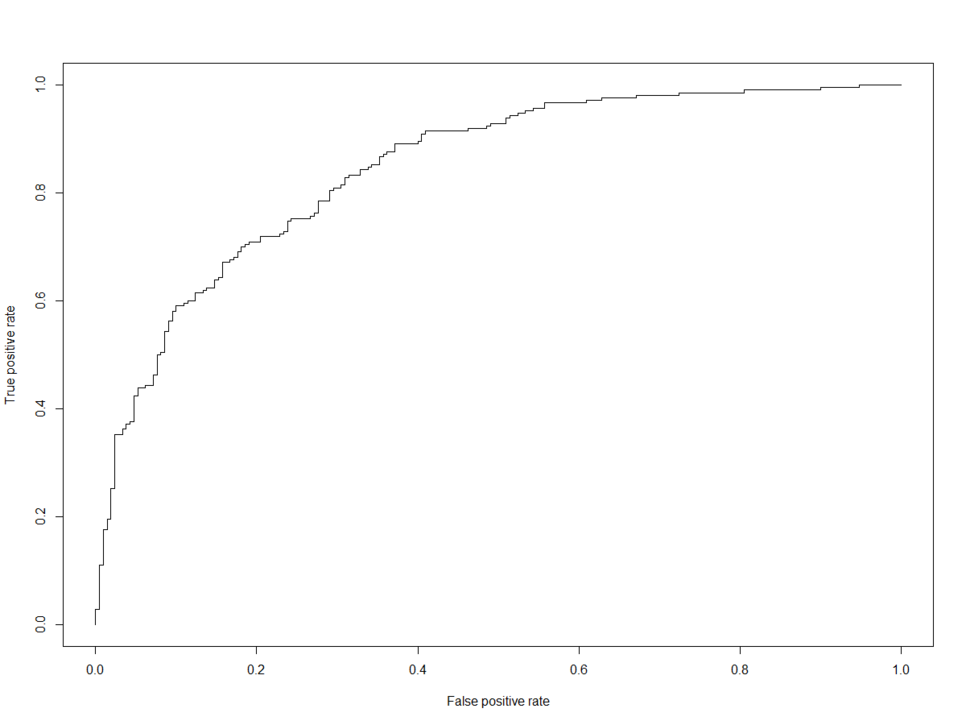
ROCR 패키지를 통해 ROC 곡선을 그릴 수 있습니다.
auc <- performance(pr, measure = "auc")
auc <- auc@y.values[[1]]
auc

[1] 0.8450794
ROC 곡선 아래의 면적인 AUC를 계산할 수 있습니다.
0.845로 굉장히 높은 값이 나왔네요.
fitted.results <- predict(log_reg,newdata=vd,type='response')
fitted.results <- ifelse(fitted.results > 0.8,'Y','N')
misclassification_valid <- mean(fitted.results != vd$Credit_status)
misclassification_valid

[1] 0.3611111
마지막으로, Test 데이터셋에 대한 오분류율도 확인해보았습니다.
'데이터 다루기 > Base of R' 카테고리의 다른 글
| [R] 연관성 분석 (Association rule) (0) | 2020.04.19 |
|---|---|
| [R] Decision Tree (의사결정나무) (0) | 2020.04.09 |
| [R] K-nearest neighbor (KNN) method (0) | 2020.04.07 |
| [R] Hierarchical clustering, K-means clustering (0) | 2020.03.16 |
| [R] Principal Component Analysis (PCA), Factor Analysis (0) | 2020.03.11 |

