논문 : Yu, T., & Zhu, H. (2020). Hyper-parameter optimization: A review of algorithms and applications. arXiv preprint arXiv:2003.05689.
3. Search Algorithms and Trial Schedulers on Hyper-Parameter Optimization
이전 포스팅에서 다룬 내용을 요약하면, 딥러닝 네트워크에서 train-related 혹은 structure-related 하이퍼파라미터는 모델의 성능에 큰 영향을 미칩니다.
본 section에서는 하이퍼파라미터 결정에 큰 도움을 줄 수 있는 탐색 알고리즘에 대해서 간략하게 리뷰해볼 예정입니다.
하이퍼파라미터는 정수, 실수, 범주형, 이진변수등의 다양한 형태를 가질 수 있으며, 이는 탐색 공간에서 분포 형태를 가집니다.
수학적으로 볼 때, HPO는 네트워크의 목적 함수로서, Loss를 최소화 하거는 Accuracy를 최대화하는 하이퍼파라미터셋을 발견하는 것입니다.
대표적인 하이퍼파라미터 탐색 알고리즘은 크게 search algorithms과 trial scheduler로 나누어집니다.
(1) Search Algorithms
A) Grid Search
Grid search는 분석자가 충분한 컴퓨팅 소스만 갖추고 있다면, 가장 정확한 하이퍼파라미터 탐색 방법이다.
모든 하이퍼파라미터의 조합에 대해서 탐색을 진행하는 방법이라고 생각하면 된다.
예를 들어서, 3개의 하이퍼파라미터에 대해서, 각 3개의 후보가 있다고 가정하면, 총 3 X 3 X 3 = 27 가지 하이퍼파라미터 셋에 대해서 전부 확인해보는 것이다.
하지만 실제로는 이를 활용하기는 매우 어렵다.
하이퍼 파라미터의 종류가 무수히 많을 뿐만 아니라, 한 번의 학습에 소모되는 시간이 데이터가 많을수록 기하급수적으로 증가하기 때문이다.
B) Random Search
Random search는 Grid search와 근본적으로 비슷하지만, 좀 더 발전된 방법이다.
위 논문에서는 Random search의 장점으로 두 가지를 설명한다.
- A budget can be assigned independently according to the distribution of search space.
- Although obtaining the optimum using random search is not promising, it is quite certain that greater time consumption will lead to a larger probability of finding the best hyper-parameter set.
하지만 Random search 또한 여전히 매우 계산 복잡한 방법이다.
C) Bayesian Optimization and its variants
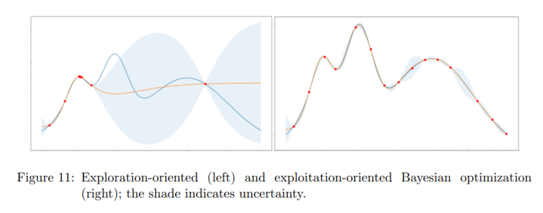
Bayesian optimization은 두 가지 절차의 밸런스 게임으로 이루어진다.
Exploitation은 현재 가지고 있는 정보로 가장 나은 결정을 내리는 절차이다.
Exploration은 정보를 더 수집하는 절차이다.
위 논문에서 설명하기를, Bayesian optimization는 두 가지 측면에서 grid search와 random search 보다 좋다고 한다.
- users are not required to possess preliminary knowledge of the distribution of hyper-parameters
- posterior probability, which is the core idea of BO
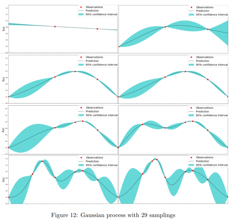
The process of BO is described as follows: a probability surrogate model of objectives is built, and then every attempt is made based on the assessment of previous trials, and furthermore, the probability model is updated for the next trial until the most promising hyper-parameter set is chosen.
BO는 두 개의 핵심 요소가 있다.
Bayesian probability surrogate model to model the objective function, and an acquisition function to determine the next sampling point.
(1) build a prior distribution of the surrogate model;
(2) obtain the hyper-parameter set that performs best on the surrogate model;
(3) compute the acquisition function with the current surrogate model;
(4) apply the hyper-parameter set to the objective function;
(5) update the surrogate model with new results.
Many probability models could be used in the BO algorithm (Eggensperger et al., 2013), but Gaussian process (GP) (Rasmussen, 2003) is overwhelmingly the most widely used. Various acquisition functions have been proposed in previous studies, including the probability of improvement (Kushner, 1964), GP upper confidence bound (GP-UCB) (Lai and Robbins, 1985; Srinivas et al., 2009), predictive entropy search (Hern´andez-Lobato et al., 2014), and even a portfolio containing multiple acquisition strategies (Hoffman et al., 2011).
BO는 머신러닝 모델에서 최적의 하이퍼파라미터를 찾는 방법으로 각광받고 있습니다.
하지만 vanilla BO에는 세 가지 치명적인 단점이 있습니다.
BO는 순차적인 방법이기 때문에, 병렬처리가 불가능합니다.
예를 들어서, 머신러닝을 10개의 컴퓨터로 처리한다고 했을 때, grid search의 경우 한 번에 10개의 경우의 수를 체크할 수 있습니다. 반면에 BO는 이전 시도를 바탕으로 진행하다보니, 반드시 1개의 경우의 수 밖에 못 사용하기 때문에 9개의 컴퓨터가 낭비됩니다.
최근에는 이러한 병렬 처리 단점을 극복한 연구들이 진행되었습니다.
A method was proposed based on the batch input of current results (Ginsbourger et al., 2011). As GP+EI is the most popular combination for Bayesian optimization, improvements based on EI (Ginsbourger et al., 2010; Snoek et al., 2012) and GP-UCB (Hutter et al., 2012; Desautels et al., 2014) Parallelization on other acquisition functions (e.g. information-based function) and the combination of BO with other algorithms (Falkner et al., 2018) are also feasible solutions.
두번째 단점으로 BO는 grid search와 random search에 비해서 계산이 복잡하다는 것입니다.
딥러닝 모델 자체로도 계산량이 엄청난데, BO까지 더해지면 감당할 수 없다는 것입니다.
이에 대한 해법으로 BO를 좀더 빠르고 자원 효율적으로 바꿔주는 연구들이 있습니다.
A straightforward method for solving this problem is to set a boundary and determine whether a certain trial is still worthy of training. This boundary could be the loss function or average accuracy in the neural network. Domhan roposed a predictive termination method that can be combined with the Bayesian method. This idea can be combined with search algorithms other than BO (Domhan et al., 2015).Freeze-thaw Bayesian optimization (Swersky et al., 2014) utilizes a forecast curve to determine whether to freeze a current trial or thaw a previous one. Currently, BO has been applied for hyper-parameter tuning in deep learning networks, which has led to achievements in both image classification (Snoek et al., 2015) and natural language processing (Melis et al., 2017).
마지막으로 BO는 실수형 하이퍼파라미터에만 적용 가능하다는 것입니다.
하지만 딥러닝 모델에서는 글 맨처음에 언급했다시피, 하이퍼파라미터는 정수형, 범주형 등의 다양한 형태를 가질 수 있습니다.
이에 대한 해법으로 surrogate 모델을 Tree structure로 구성하는 방법이 있습니다.
Tree-structured Parzen Estimators 는 다음 섹션에서 크게 다뤄보도록 하겠습니다.
D) Tree Parzen Estimators (TPEs)
TPEs는 시각적 구조를 가지며, 이는 conditional search space를 다루기 위한 surrogate model로 사용됩니다.
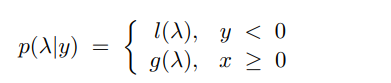
In summary, the workflow of TPE is as follows: draw a sample from l(x), evaluate l(x)/g(x) with EI, and obtain the optimum value of l(x)/g(x) with the greatest EI. TPE outperforms the Bayesian method in dealing with conditional variables because of its tree structure (Strobl et al., 2008).
(2) Optimization with an Early-stopping Policy
HPO는 계산 비용이 매우 큰, 시간 소모적인 작업입니다.
실제 데이터에서는 하이퍼파라미터 튜닝을 완전하게 하기에는 현실적인 한계에 부딪힙니다.
전문가들은 도메인 지식을 활용해서 하이퍼파라미터 탐색 공간을 좁힐 수 있습니다.
Early stopping 전략은 모델 자체에서 AI Expert를 흉내내도록 도와줍니다.
A) Median Stopping
Median stopping은 매우 직관적인 early stopping 기법입니다. 현재 Google Vizier (Golovin et al., 2017), Tune (Liaw et al., 2018), and NNI (Microsoft, 2018) 등에 채택되어 있습니다.
Median stopping makes a decision based on the average of primary metrics (e.g., accuracy or loss) reported by previous runs. A trial X is stopped at step S if the best objective value by step S is strictly worse than the median value of the running average of all completed trials objective values reported at step S (Golovin et al., 2017).
B) Curve Fitting
Curve fitting은 LPA (learning, predicting, assessing) 알고리즘 중 하나입니다.
This early stopping rule makes a prediction of the final objective value (e.g., accuracy or loss) with a performance curve regressed from a set of completed or partially completed trials. A trial X will be halted at step S if the prediction of the final objective value is sufficiently worse than the tolerant value of the optimal in the trial history.

'데이터 다루기 > 머신러닝 이론' 카테고리의 다른 글
| 하이퍼 파라미터 튜닝 (1) (0) | 2021.11.22 |
|---|---|
| [Machine Learning] XGBoost (3) Optimization technique (0) | 2020.10.05 |
| [Machine Learning] XGBoost (2) Methematical details (0) | 2020.10.05 |
| [Machine Learning] XGBoost (1) Algorithm Schema (0) | 2020.10.05 |
| [Machine Learning] Gradient Boosting (Classification) (0) | 2020.09.27 |


